Example f″(x) = 0 IS an Inflection Point.

Determine the intervals where the function is concave up and concave down, and the location of any inflection points.

$f\left(x\right)=3x^5–20x^3$

Step 1: Find the 2 ^nd Derivative, $f\prime \prime \left(x\right)$.

$f\left(x\right)=3x^5–20x^3$

$f\prime \left(x\right)=15x^4–60x^2$

$f\prime \prime \left(x\right)=60x^3–120x$

Step 2: Find the location of the possible inflection points where $f\prime \prime \left(x\right)=0$ or $f\prime \prime \left(x\right)= \mathit{Does\; Not\; Exist }\left(\mathit{DNE}\right)$

In this situation you do not need to concern yourself with the $f\prime \prime \left(x\right)= \mathit{Does\; Not\; Exist }\left(\mathit{DNE}\right)$ scenario because there are no fractions, and no other places that math would “break”.

Algebra Moves:

i)  Factor a 60x out of the equation.

ii) Separate it into two math problems with both pieces being set equal to zero.

iii) First, on the left column you will isolate the x , by dividing both sides by 60.

iv) On the right column you will isolate the $x^2$, and then take the square root of both sides to solve for x . Remember when you apply the square root, you get the $\pm$ of that result, not just the positive.

$f\prime \prime \left(x\right)=60x^3–120x$

$0=60x^3–120x$

$0=60x\left(x^2–2\right)$

$0=\mathrm{ }60x$

$\frac{0}{60}=\frac{60x}{60}$

$0=x$

${\overline{)0=x}}^{\mathit{Possible\; Inflection\; Point}}$

$0=x^2–2$

$\begin{array}{c}0\\ \underline{+2}\end{array}=\begin{array}{c}{x}^2–2\\ \underline{+2}\end{array}$

$2=x^2$

$\sqrt{2}=\sqrt{x^2}$

$\pm \sqrt{2}=x$

$–\sqrt{2}=\mathit{x }\mathrm{and }\sqrt{2}=x$

${\overline{)–\sqrt{2}=\mathit{x } }}^{\mathit{Possible\; Inflection\; Point}}$and ${\overline{)\sqrt{2}=x }}^{\mathit{Possible\; Inflection\; Point}}$

Step 3: Do the 2 ^nd Derivative Test (number line game)

i) Draw a number line.

If you are provided an x-interval , [ a , b ], make those endpoints the ends of your number line.

ii) Mark all of your possible inflection points on the number line.

iii) Choose test values on either side (left and right) of your possible inflection points , and mark them on the number line.

iv) Do the actual 2 ^nd Derivative Test.

Plug your test values into your 2 ^nd Derivative, $f\prime \prime \left(x\right)$. Remember math people are not creative namers. It is called the 2 ^nd Derivative Test because you are testing everything in the 2 ^nd Derivative, $f\prime \prime \left(x\right)$.

v) Mark the results either positive (concaveup) or negative (concave down) on your number line.

Include a drawing of the concavity that goes with that behavior.

i)

ii)

iii)

iv) $f\prime \prime \left(x\right)=60x^3–120x$

$f\prime \prime \left(–3\right)=60{\left(–3\right)}^3–120\left(–3\right)=–1260 \left(\mathit{negative}\right)$

$f\prime \prime \left(–1\right)=60{\left(–1\right)}^3–120\left(–1\right)=60 \left(\mathit{positive}\right)$

$f\prime \prime \left(1\right)=60{\left(1\right)}^3–120\left(1\right)=–60 \left(\mathit{negative}\right)$

$f\prime \prime \left(3\right)=60{\left(3\right)}^3–120\left(3\right)=1260 \left(\mathit{positive}\right)$

v)

Step 4a Draw Conclusions: Intervals where the original equation, $f\left(x\right)$, is concave up and concave down.

You will read this information directly from your 2 ^nd Derivative Test number line. This is why I really like to draw the shape of the concavity on the number. It just makes reading the data off that much easier.

Intervals where $f\left(x\right)$ is concave up, you want to find the intervals on your 2 ^nd Derivative number line where the value is positive, where you have a concave up shape drawn. Here you have a positive 2 ^nd Derivative starting at an inflection point $x=–\sqrt{2}$and ending at your inflection point of $x=0$. And again, starting at your inflection point of $x=\sqrt{2}$ and going on to $\infty$.

Intervals where $f\left(x\right)$ is concave down, you want to find the intervals on your 2 ^nd Derivative number line where the value is negative, where you have a concave down shape. Here you have a negative 2 ^nd Derivative starting on the left at $–\infty$and ending at the inflection point$x=–\sqrt{2}$. It then starts again at your inflection point of $x=0$ and ends at the inflection point $x=\sqrt{2}$.

Remember that at your actual inflection point the 2 ^nd Derivative equals 0, $f\prime \prime \left(x\right)=0$. This means the graph is not concave up or concave down at that moment. You will not want to include those x-values in the interval, which means you will want to use parenthesis in your interval notation.

Step 4a Draw Conclusions: Location of the inflection points.

Check if the second requirement to be an inflection point is met.

2)      The function, $f\left(x\right)$, must change concavity at that point.

If that second requirement is met, then you need to plug that x-value back into the original equation, $f\left(x\right)$, to determine y-value that goes with it. An inflection point means you need the full point, ( x , y ).

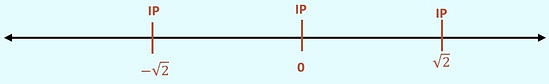
In this example you have 3 possible inflection points:

$x=–\sqrt{2},0,\mathrm{ }\sqrt{2}\mathrm{ }$

At $x=–\sqrt{2}$, the concavity switches from negative to positive. It IS an inflection point.

At $x=0$, the concavity switches from positive to negative. It IS an inflection point.

At $x=\sqrt{2}$, the concavity switches from negative to positive. It IS an inflection point.

Finally, you need to plug those x-values back into the original equation, $f\left(x\right)$, to get the y-values that go with them.

Step 4a Draw Conclusions: Intervals where the original equation, $f\left(x\right)$, is concave up and concave down.

The original function, $f\left(x\right)=3x^5–20x^3$, is concave up on the x-interval $\left(–\sqrt{2},0\right)\cup \left(\sqrt{2},\mathrm{\infty }\right)$.

The original function, $f\left(x\right)=3x^5–20x^3$, is concave down on the x-interval $\left(–\mathrm{\infty },–\sqrt{2}\right)\cup \left(0,\sqrt{2}\right)$.

Step 4a Draw Conclusions: Location of the inflection points.

Original Function: $f\left(x\right)=3x^5–20x^3$

Inflection point: $f\left(–\sqrt{2}\right)=3{\left(–\sqrt{2}\right)}^5–20{\left(–\sqrt{2}\right)}^3=28\sqrt{2}$

Inflection point: $f\left(–\sqrt{2}\right)=28\sqrt{2}$

Inflection point:  $\left(–\sqrt{2},28\sqrt{2}\right)$

Inflection point: $f\left(0\right)=3{\left(0\right)}^5–20{\left(0\right)}^3=0$

Inflection point:  $f\left(0\right)=0$

Inflection point: $\left(0,0\right)$

Inflection point:  $f\left(\sqrt{2}\right)=3{\left(\sqrt{2}\right)}^5–20{\left(\sqrt{2}\right)}^3=–28\sqrt{2}$

Inflection point: $f\left(\sqrt{2}\right)=–28\sqrt{2}$

Inflection point:  $\left(\sqrt{2},–28\sqrt{2}\right)$

Final Result:

The function $f\left(x\right)=3x^5–20x^3$ has three inflection points at $\left(–\sqrt{2},28\sqrt{2}\right), \left(0,0\right), \mathrm{and }\left(\sqrt{2},–28\sqrt{2}\right)$.

The function $f\left(x\right)=3x^5–20x^3$is concave up on the x-interval $\left(–\sqrt{2},0\right)\cup \left(\sqrt{2},\mathrm{\infty }\right)$.

The function $f\left(x\right)=3x^5–20x^3$, is concave down on the x-interval $\left(–\mathrm{\infty },–\sqrt{2}\right)\cup \left(0,\sqrt{2}\right)$.