Example 2: f′(x) = 0 on Closded Interval [a,b]

Determine all relative extrema and the intervals where the function is increasing and decreasing on the interval [-4,4].

$f\left(x\right)=3x^5–20x^3$

Step 1: Find the 1 ^st Derivative, $f^{\prime }\left(x\right)$.

$f\left(x\right)=3x^5–20x^3$

$f\prime \left(x\right)=15x^4–60x^2$

Step 2: Find the critical values of the equation.

$f^{\prime }\left(x\right)=0$ OR $f^{\prime }\left(x\right)= \mathit{Does\; Not\; Exist }\left(\mathit{DNE}\right)$

In this situation you have a closed interval, [-4,4], so the endpoints of the interval are locations where $f^{\prime }\left(x\right)= \mathit{Does\; Not\; Exist }\left(\mathit{DNE}\right)$. This gives us two critical values that we must include in our 1 ^st Derivative Test.

Now to find the places where $f^{\prime }\left(x\right)=0$, all that is needed is to take the derivative and set it equal to zero, then solve that equation for x . Most times when you set an equation equal to zero, the algebraic method for solving it is the same. Factor the equation and then set those smaller equations equal to zero, and find their solutions.

Algebra Moves:

i)  Factor a $15x^2$ out of the equation.

ii) Separate it into two math problems with both pieces being set equal to zero.

iii) First, in the left column we will isolate the $x^2$. Start by dividing both sides by $15$,and then take the square root of both sides to solve for x .

iv) Next, in the right column we will again isolate the $x^2$, and then take the square root of both sides to solve for x . Remember when you apply the square root , you get the $\pm$ of that result, not just the positive.

$f^{\prime }\left(x\right)= \mathit{Does\; Not\; Exist }\left(\mathit{DNE}\right)$

Closed interval, [-4,4]

${\overline{)x=–4}}^{\mathit{Critical\; Value}} \mathit{and }{\overline{)x=4 }}^{\mathit{Critical\; Value}}$

$f^{\prime }\left(x\right)=0$

$0=15x^4–60x^2$

$0={15x}^2\left(x^2–4\right)$

$0={15x}^2$

$\frac{0}{15}=\frac{{15x}^2}{15}$

$0=x^2$

$\sqrt{0}=\sqrt{x^2}$

$0=x$

${\overline{)0=x}}^{\mathit{Critical\; Value}}$

$0=\left(x^2–4\right)$

$\begin{array}{c}0\\ \underline{+4}\end{array}=\begin{array}{c}{x}^2–4\\ \underline{+4}\end{array}$

$4=x^2$

$\sqrt{4}=\sqrt{x^2}$

$\pm 2=x$

$–2=\mathit{x }\mathit{and }2=x$

${\overline{)–2=x}}^{\mathit{Critical\; Value}} \mathit{and }{\overline{)2=x\mathrm{ }}}^{\mathit{Critical\; Value}}$

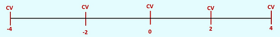
Step 3: Do the actual 1 ^st Derivative Test (number line game).

i)                     Draw a number line.

ii)                   Mark all of your critical values on the number line.

iii)                 Choose test values on either side (left and right) of your critical values , and mark them on the number line.

iv)                 Do the actual 1 ^st Derivative Test. Plug your test values into your 1 ^st Derivative, $f\prime \left(x\right)$. Remember math people are not creative namers. It is called the 1 ^st Derivative Test it is because you are testing everything in the 1 ^st Derivative, $f\prime \left(x\right)$.

v)                   Mark the results either positive (increasing) or negative (decreasing) on your number line. Including drawing the directional arrow that goes with that behavior.

i)                      

ii)                    

iii)                  

iv)                 $f\prime \left(x\right)=15x^4–60x^2$

$f\prime \left(\mathit{–}\mathit{3}\right)=15{(\mathit{–}\mathit{3})}^4–60{(\mathit{–}\mathit{3})}^2=675 \left(\mathit{positive}\right)$

$f\prime \left(\mathit{–}\mathit{1}\right)=15{(\mathit{–}\mathit{1})}^4–60{(\mathit{–}\mathit{1})}^2=–45 \left(\mathit{negative}\right)$

$f\prime \left(\mathit{1}\right)=15{\left(\mathit{1}\right)}^4–60{\left(\mathit{1}\right)}^2=–45 \left(\mathit{negative}\right)$

$f\prime \left(\mathit{3}\right)=15{\left(\mathit{3}\right)}^4–60{\left(\mathit{3}\right)}^2=675 \left(\mathit{positive}\right)$

v)                    

Step 4a Draw Conclusions : Relative Extrema

Reading off the relative extrema is really why I like drawing the directional arrows on the number line.

When you look for a relative maximum, we want to see the shape of a max  .

When you look for a relative minimum, we want to see the shape of a min .

Looking at the three critical values that are not your endpoints, you can see that you have a relative maximum occurring at x = -2 , a relative minimum occurring at x = 2 , and neither a max or min occurring at x = 0 . Just because you have a critical value does not mean that that value is a max or min.

Now looking at the two critical values that are your endpoints, x = -4 and x = 4 , you must think a bit more about the behavior that is occurring.

Looking at x = -4 you see that every value from there would be up, increasing.

That means locally, in its neighborhood, at x = -4 there would be a relative minimum.

Looking at x = 4 you see that every value coming into the endpoint would be going up, increasing. The highest point would be at then end of that increase, the endpoint, x = 4 .

That means locally, in its neighborhood, at x = 4 would be a relative maximum.

The final move is to now plug those x-values back into the original equation, $f\left(x\right)$. This will tell you what the actual max or min y-value is.

Step 4b Draw Conclusions: Intervals where the original equation, $f\left(x\right)$, is increasing and decreasing.

You will read this data directly from your 1 ^st Derivative Test number line . This is why I really like to draw the directional arrows on that number line.

Intervals on your 1 ^st Derivative Test number line where the derivative, $f\prime \left(x\right)$, value is positive, where you have an arrow pointing up are the increasing intervals .

Here you have a positive derivative starting at the left endpoint x = -4 and ending at the critical value of x = -2 . And starting again at your critical value of x = 2 and ending at the right endpoint of x = 4 .

Intervals on your 1 ^st Derivative Test number line where the derivative, $f\prime \left(x\right)$, value is negative, where you have an arrow pointing down are the decreasing intervals .

Here you have a negative derivative starting at your critical value of x = -2 and ending for just an instant at the critical value x = 0 . It then starts again at your critical value of x = 0 and ends at the critical value x = 2 .

You need to break the interval into two pieces because at the critical value , x = 0 , the graph is not increasing or decreasing.

Step 4a Draw Conclusions : Relative Extrema

$f\left(x\right)=3x^5–20x^3$

Local Min: $f\left(–4\right)=3{\left(–4\right)}^5–20{\left(–4\right)}^3=–1792$

Local Min: $f\left(–4\right)=–1792$

Local Max: $f\left(–2\right)=3{\left(–2\right)}^5–20{\left(–2\right)}^3=64$

Local Max: $f\left(–2\right)=64$

Local Min: $f\left(2\right)=3{\left(2\right)}^5–20{\left(2\right)}^3=–64$

Local Min: $f\left(2\right)=–64$

Local Max: $f\left(4\right)=3{\left(4\right)}^5–20{\left(4\right)}^3=1792$

Local Max: $f\left(4\right)=1792$

Step 4b Draw Conclusions: Intervals where the original equation, $f\left(x\right)$, is increasing and decreasing.

The original function, $f\left(x\right)=3x^5–20x^3$, is increasing on the x-interval $\left(–4,–2\right)\cup \left(2,4\right)$.

The original function, $f\left(x\right)=3x^5–20x^3$, is decreasing on the x-interval $\left(–2,0\right)\cup \left(0,2\right)$.

Final Result:

The function $f\left(x\right)=3x^5–20x^3$ has a relative min of y = -1792 at x = -4 .

The function $f\left(x\right)=3x^5–20x^3$ has a relative max of y = 64 at x = -2 .

The function $f\left(x\right)=3x^5–20x^3$ has a relative min of y = -64 at x = 2 .

The function $f\left(x\right)=3x^5–20x^3$ has a relative max of y = 1792 at x = 4 .

The function $f\left(x\right)=3x^5–20x^3$is increasing on the x-interval $\left(–4,–2\right)\cup \left(2,4\right)$.

The function $f\left(x\right)=3x^5–20x^3$, is decreasing on the x-interval $\left(–2,0\right)\cup \left(0,2\right)$.