Method: Area Between Two Curves

The setup for these problems is really the key to the whole thing. Once you have your integral setup, you only need to run the standard Definite Integral process.

Step 1: Determine whether your equation is in terms of x (standard: $y=x^2+3x+\sqrt{x}$) or in terms of y (non-standard: $x=y^2+3y+\sqrt{y}$).

This is one of the few times in AP Calculus that you have to consider the graphical changes that occur when you change the independent variable . The reason it is important is that your Area Between Two Curves setup requires you to know which of your equations is on top and which one is on bottom, and how you visualize those will change depending upon which variable your equation is “ in terms of ”, x or y .

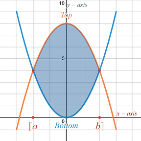
Standard setup with equations in terms of x , dx . The majority of equations you have seen to this point will have been in the form of a y = x ’s (i.e., $y=\sqrt{x}$). I know that you have used different variables, especially with “real-world” problems, but they have always been of the format where the x-axis is the independent variable (what you plug in ), and the y-axis is the dependent variable (what you get out ). 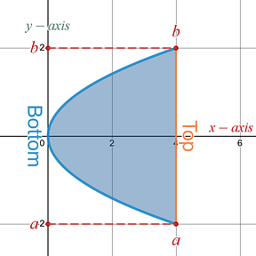$\underset{a}{\overset{b}{\int }}\mathit{Top}–\left(\mathit{Bottom}\right) \mathit{dx}$	New setup with equations in terms of y , dy . For the first time in the AP Calc course, they start introducing situations where the y-variable is the independent variable (what you plug in ), and the x-variable is the dependent variable (what you get out ). You have equations now where x = y ’s (i.e., $x=y^2+2y–7$).   As you try to determine which equation is on top on bottom, I have found it useful to physically rotate my book, paper, or calculator 90 ◦ to the left (counter clockwise) when first learning the process. Some people are great at doing these types of rotations in their heads, and you will be able to too after some practice. When you first start though you might want to try it.
	Standard: Not Rotated x-axis running left and right y-axis running up and down	Rotated left 90 ◦ x-axis is running up and down y-axis is running left and right
	$\underset{a}{\overset{b}{\int }}\mathit{Top}–\left(\mathit{Bottom}\right) \mathit{dy}$

 

Step 2: Determine the bounds of the integral, $\underset{a}{\overset{b}{\int }}$, for each of your enclosed regions.

• Your bounds are either going to be the intersection of your two equations, or they will be defined by an equation you were given.

Intersections as Bounds

Equations as Bounds

 

• If you are given an actual graph to work from, then you should be able to just read the bounds of your integral straight off the graph.
• If you are given equations and allowed to use your calculator, then you will be able to calculate the intersects of your two graphs using the Calc–Intersect function on your TI-84 calculator.
• When the region is closed off (bounded) on the left and right side by additional given equations which are vertical lines (i.e., x=2 , x=5 ), then those vertical lines will create your bounds.
• Sometimes you will be given only the equations, you will not be allowed to use your calculator, and you will have to calculate the intersects of those two equations by setting the two equations equal to each other and solving for the intersects (solving for x ).

Step 3: Determine the Top and Bottom equations for all of your enclosed regions.

• Most of the time on the actual AP Calc Exam, these problems provide you the graphs to work from. In those situations, you need to look at the given graphs, choose the Top equation based on the graph that is above (larger y-values ) the other graph, the Bottom equation.
• If you are not given the graph, you are often times allowed to use your TI-84 calculator to graph the given equations. Graph the two equations on your TI-84 calculator and again visually determine the Top and Bottom from that graph.
• If you do not have either of the previous two options available to you, then you are going to need to sketch the graphs yourself. These equations will most likely come from your standard family of graphs.

The short list of graphs you should be able to sketch a graph on your own would be:

• Linear ($y=\mathit{mx}+b$)
• Quadratic or Parabolas ($y=x^2$)
• Cubic ($y=x^3$)
• Square root ($y=\sqrt{x}$)
• Exponential ($y=a\bullet b^x$)
• Sine ($y=\mathit{sin}\left(x\right)$)
• Cosine ($y=\mathit{cos}\left(x\right)$)
• Vertical lines ($x=5$)

That is not an exhaustive list, but will give you a good starting point.

• The method of last resort would be to do a plug and chug process.
  • Choose a test x-value from each of your region’s x-interval .

Create a number line broken into regions based upon the intersections or bounds that you found in Step 2 .  (Think number line like a 1 ^st Derivative Test). Choose a test x-value from each of the regions you have laid out.

• Plug that x-value into each of your equations to see which one chugs out the larger y-value .

The larger y-value represents the graph that is on Top because its y-value is larger than ( above ) the other equation’s y-value .

• REMEMBER: That your graphs can flip position. Which means that the graph that is on Top to start could switch position and be on Bottom later, and you will need to identify all of those changes of position. When these changes occur, you must setup a different Definite Integral for each different enclosed region.

Step 4: Setup a Definite Integral problem for each of your enclosed regions using your Area Between Two Curves formula :

$\underset{a}{\overset{b}{\int }}\mathit{Top}–\left(\mathit{Bottom}\right)\mathit{dx}=\mathit{Area\; Betwen }2\mathit{ Curves}$

Remember if you have multiple regions, then you will need to add up all those results to get your final answer for the Total Area Enclosed.