Example 1: Upper and Lower Riemann Sums
Since the only part of the Riemann Sums Method that changes from type to type is Step 5 . I will use a single equation to show you how Step 5 varies for each type of Riemann Sum.
|
Use 6 subintervals to estimate the area between the curve and the x-axis for on the interval [1,3]. Do this as an upper sum and lower sum. |
|||||
|
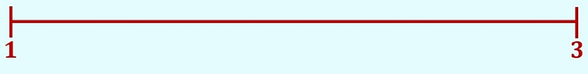
Step 1: Draw a number line with the left and right endpoints of the number line coming from your given interval, [ a , b ].
The number line will be the same for all of the methods. The interval in these problems is [1,3].
|
|
||||
|
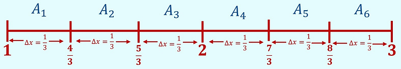
Step 2: Calculate your , the base from your formula, using the formula:
The number of intervals would be 6 since the problem asks us to use 6 subintervals. |
|
||||
|
Step 3: Mark your subintervals on your number line.
Here you have . Starting at the left endpoint and ending at the right endpoint.
Label these gaps between each mark . |
|
||||
|
Step 4: Start laying out your area formulas for each of your subintervals. |
|
||||
|
Step 5 ( ONLY STEP THAT CARES WHAT TYPE of Riemann Sum ): Choose your evaluation points, , based on the directions of your specific problem, either left, right, middle, upper, or lower.
|
For an upper sum look at each subinterval and choose the evaluation point, ,that would provide you the largest height , the largest , for that subinterval.
|
For a lower sum look at each subinterval and choose the evaluation point, ,that would provide you the smallest height , the smallest , for that subinterval.
|
|||
|
Step 6: Get your actual area value for each of your different area formulas by plugging your evaluation points, , into the actual equation, , to find your height , and then multiply those values by your , your base , to find the area, .
You use the same as the base for each of the 5 options, and we also use the same equation, , to find the heights . |
|
|
|||
|
Step 7: Add up the areas of all of your subinterval rectangles to get an estimate for the total area between the curve and the x-axis .
|
|
|
|||
|
Step 8 (only if asked): Draw the rectangles for each subinterval that you just found the areas of. Start on the x-axis at the evaluation point, , that you chose for each subinterval in Step 5 . Draw up or down from that point until you hit your actual graph, , then draw a horizontal line at that point that covers that rectangle’s subinterval, and then draw back to the x-axis . Repeat the process for each of your subintervals. I always say, “Draw up. Draw over. Draw down.”
|
|
|
|||