Riemann Sums Overview
You spend the one-third of your AP Calc course talking about derivatives. So, it makes sense to spend the last one-third of your AP Calc course learning how to undo derivatives (antiderivatives), and the applications of antiderivative techniques.
Unlike with derivatives where they teach the mechanics of the process first (i.e., power rule, product rule), and then throw you into the application (i.e., 1 st Derivative Test); with integrals or antiderivatives, they decide to throw you head first into an application of the tool. Then they teach you the mechanics after that. Why they choose to order the material this way, I have no idea, but because they do, I will also.
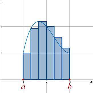
One of the applications of an integral allows you to use it to determine the area between a curve, , and the x-axis . You are introduced to this area between a curve and the x-axis application through Riemann sums. Riemann sums are a method to estimate the area between a curve and the x-axis . The Riemann sums application is the long way of estimating an integral.You learn this before you learn some very useful integration rules (i.e., power rule) to find the exact area between a curve and the x-axis in a much quicker and easier way.
Your instructor and the AP Calc team use Riemann Sums to show you the back ground for how the integral was developed.
|
Riemann Sum vs. Integral |
|
|
Riemann Sum Uses shapes (usually rectangles, but could be any shape) to estimate the area between a curve and the x-axis on a given x-interval [ a , b ]. |
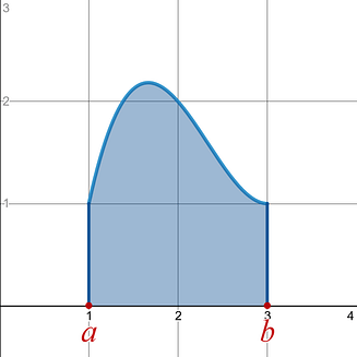
Integral Uses integration rules to find the exact area between a curve and the x-axis on a given x-interval [ a , b ]. |
|
|
|
|
Note: When considering the area between a curve and the x-axis , you will want to treat area above the x-axis as positive area, and area below the x-axis as negative area.
|
|